in nutshell
<center>


</center>
reference - http://www.mrexcel.com/forum/excel-questions/5129-vlookup-copying-formula-down-whole-column.html#post22660
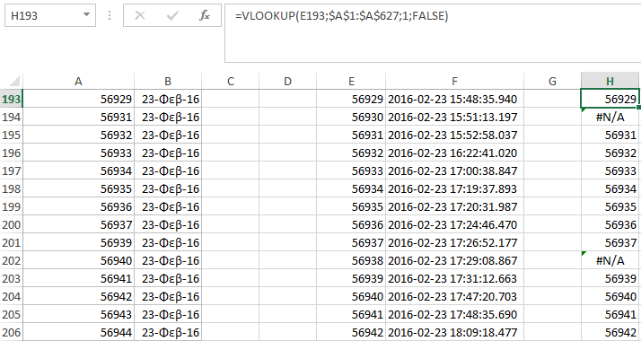
E193 = is the column with fewer values.
A1:A627 = is the column with most values.
1 = the column number in table from which the matching value must be returned. The first column is 1.
FALSE = (Optional) Enter FALSE to find an exact match. Enter TRUE (default) to find an approximate match.
the $sign take place when dragging the first cell dont change this value
create the formula on top cell then drag it till bottom
or use
End of Excel VLOOKUPS – Power Pivot Relationships
https://blogs.msdn.microsoft.com/microsoft_press/2016/03/16/from-the-mvps-end-of-excel-vlookups-power-pivot-relationships/
<center>
</center>
reference - http://www.mrexcel.com/forum/excel-questions/5129-vlookup-copying-formula-down-whole-column.html#post22660
JavaScript:
=VLOOKUP(E193;$A$1:$A$627;1;FALSE)E193 = is the column with fewer values.
A1:A627 = is the column with most values.
1 = the column number in table from which the matching value must be returned. The first column is 1.
FALSE = (Optional) Enter FALSE to find an exact match. Enter TRUE (default) to find an approximate match.
the $sign take place when dragging the first cell dont change this value
create the formula on top cell then drag it till bottom
or use
JavaScript:
//compare A1 with B1
=A1=B1
End of Excel VLOOKUPS – Power Pivot Relationships
https://blogs.msdn.microsoft.com/microsoft_press/2016/03/16/from-the-mvps-end-of-excel-vlookups-power-pivot-relationships/